dexterMST: dexter for Multi-Stage Tests
Timo Bechger, Jesse Koops, Robert Zwitser, Ivailo Partchev, Gunter Maris
2018-07-13
Source:vignettes/blog/2018-07-13-dextermst.Rmd
2018-07-13-dextermst.RmddexterMST is a new R package acting as a companion to dexter (Maris et al. 2018) and adding facilities to manage and analyze data from multistage tests (MST). It includes functions for importing and managing test data, assessing and improving the quality of data through basic test and item analysis, and fitting an IRT model, all adapted to the peculiarities of MST designs. It is currently the only package that offers the possibility to calibrate item parameters from MST using Conditional Maximum Likelihood (CML) estimation (Zwitser and Maris 2015). dexterMST will accept designs with any number of stages and modules, including combinations of linear and MST. The only limitation is that routing rules must be score-based and known before test administration.
What does it do?
Multi-stage tests (MST) must be historically the earliest attempt to achieve adaptivity in testing. In a traditional, non-adaptive test, the items that will be given to the examinee are completely known before testing has started, and no items are added until it is over. In adaptive testing, the items asked are, at least to some degree, contingent on the responses given, so the exact contents of the test only becomes known at the end. (Bejar 2014) gives a nice overview of early attempts at adaptive testing in the 1950s. Other names for adaptive testing used in those days were tailored testing or response-contingent testing. Note that MST can be done without any computers at all, and that computer-assisted testing does not necessarily have to be adaptive.
When computers became ubiquitous, full-scaled computerized adaptive testing (CAT) emerged as a realistic option. In CAT, the subject’s ability is typically reevaluated after each item and the next item is selected out of a pool, based on the interim ability estimate. In MST, adaptivity is not so fine-grained: items are selected for administration not separately but in bunches, usually called modules. In the first stage of a MST, all respondents take a routing test. In subsequent stages, the modules they are given depend on their success in previous modules: test takers with high scores are given more difficult modules, and those with low scores are given easier ones – see e.g., Zenisky et al. (2009), Hendrickson (2007), or Yan et al. (2014).
Hence, MST can be seen as middle ground between CAT and linear testing, and can be approached from either side: as a CAT that has been somewhat coarsened, or as adding adaptivity to the more traditional designs. We prefer to go the latter way because our experience is so much larger with linear, multi-booklet designs.
Below is a schematic representation of the data from a very simple, linear, one-booklet test. We assume that the columns have been sorted by increasing item difficulty, and the rows have been sorted by increasing person ability.
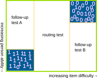
Note the two corners that have been highlighted in blue. When we ask very easy items to very able examinees, the responses are quite predictable, and hence not very informative. Most will be correct, and the few wrong ones might be due to momentary lapse of attention (slipping). When we ask difficult items to less able examinees, the result is the opposite yet similar, and the few correct responses might be attributed to lucky guessing.
What if we simply refuse to collect this worst, least informative part of the data? We end up with something akin a very simple MST. The central part that has been given to all examinees may be regarded as a routing test, and the two incomplete parts as the follow-up modules: A for the less able examinees, B for the others. If we don’t ask items that are much too easy or much too difficult for the examinee, we avoid demotivation and frustration, correspondingly, and with them much of the motivation to approach the data with a 3- or 4-parameter IRT model. It seems preferable to downsize slipping and guessing physically than to try to accommodate them mathematically.
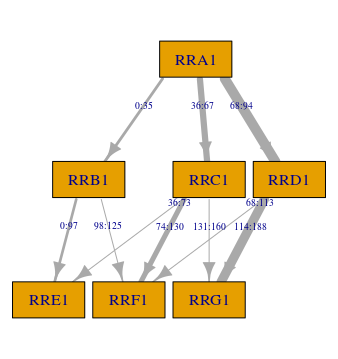
This is a somewhat primitive and not entirely accurate example – for example, the routing test does not have to be confined to items of average difficulty. Still, it explains some of the basic motivation for adaptivity and MST. To get closer to actual work with MST, it is more convenient to represent the test design with a tree diagram. A very simple example is shown below:

The tree is read from top to bottom. The root represents the first stage where all examinees take the first module (the routing test). In the second stage, examinees with a score lower than or equal to 5 on the routing test take module 2, whereas examinees with a score higher than 5 on the routing test take module 3. Every path corresponds to a booklet. In this MST, there are two booklets: the first one, booklet M1-M2, should be relatively easy while the other, M1-M3, is more difficult.
Unlike CAT, MST is not all about algorithms. Most concepts, steps, procedures known from linear testing and familiar from dexter are still in place, but in a modified form: some are a bit more complicated, others quite a bit, a few become meaningless. We next review the basic workflow, which is similar to dexter with a few important additions, and we discuss some of the differences in more detail.
How do I use it?
There are not too many workflows to manage and analyze test data. In dexter, the procedure is, basically:
- Start a project
- Declare the scoring rules for all items
- Input data
- Examine data, assess quality with classical statistics, make necessary adjustments
- Estimate item parameters
- DIF, profile analysis …
- Estimate and analyze proficiencies
In dexterMST, we follow more or less the same path except that we must, between steps 2 and 3, communicate the MST structure to the program: the modules, the booklets, and the routing rules.
Create a MST project
The first step in dexterMST is to create a new project (actually, an empty data base). In this example, the project is created in memory, and it will be lost when you close R. To create a permanent project, simply replace the string “:memory:” by a file name.
db = create_mst_project(":memory:")Supply the scoring rules
Just like in dexter, the first really important step
is to supply the scoring rules: an exhaustive list of all items
that will appear in the test, all admissible responses, and the score
that will be assigned to each response when grading the test. These must
be given as a data.frame with three columns: item_id,
response and item_score: the first two are
strings, and the scores are integers with always 0 as the lowest
possible score.
Note that the three column names must be exactly as shown above. We could have allowed for arbitrary names but, since variable names play an important role in entering data, we thought that a bit of extra discipline would not be excessive in this particular case.
If you have scored data, you can simply make the column response match the item_score, as in the following example:
| item_id | response | item_score |
|---|---|---|
| item01 | 0 | 0 |
| item01 | 1 | 1 |
| item02 | 0 | 0 |
| item02 | 1 | 1 |
| item03 | 0 | 0 |
| item03 | 1 | 1 |
| item04 | 0 | 0 |
| item04 | 1 | 1 |
add_scoring_rules_mst(db, scoring_rules)Define the test design
In the simpler case of multi-booklet linear tests, dexter is able to infer the test design from the scoring rules and the test data. With MST, we have to work some more and provide information on the modules and the routing rules.
First, the modules. Create another data.frame with
columns module_id, item_id and
item_position:
| module_id | item_id | item_position |
|---|---|---|
| Mod_2 | item01 | 1 |
| Mod_2 | item02 | 2 |
| Mod_2 | item03 | 3 |
| Mod_2 | item04 | 4 |
| Mod_2 | item05 | 5 |
| Mod_2 | item06 | 6 |
| Mod_2 | item07 | 7 |
| Mod_2 | item08 | 8 |
Note that the items have been sorted in difficulty which is why module 2 contains the first items.
Routing rules specify the rules to pass from one
module to the next. We have supplied a function, mst_rules,
which lets you define the routing rules using a simple syntax. The
following example defines two booklets (remember, booklets are paths)
called “easy” and “hard”. The “easy” booklet consists of the routing
test, here called Mod_1, and module Mod_2; it
is given to examinees who scored between 0 and 5 on the routing test.
Booklet “hard” consists of the routing test and module
Mod_3, and is given to examinees who scored between 6 and
10 on the routing test. Obviously, the command language is a simple
transcription of the tree diagram on the previous illustration: read
--+ as arrow from left to right and [0:5] as a
score range, here from zero up to and including five.
routing_rules = mst_rules(
  easy = Mod_1[0:5] --+ Mod_2,
  hard = Mod_1[6:10] --+ Mod_3)
Having defined the two crucial elements of the design, the modules
and the routing rules, use function create_mst_test to
combine them and give the test a name, in this case
ZwitserMaris:
create_mst_test(db,
                test_design = design,
                routing_rules = routing_rules,
                test_id = 'ZwitserMaris')
Enter test data
With the test defined, you can enter data. This can be done in two ways: booklet per booklet in wide form, or all booklets at once. The former is illustrated below; the latter works if the data is in long format (also called normalized or tidy, see (Wickham and Grolemund 2017)).
| person_id | item01 | item02 | item03 | item04 | item05 | item06 |
|---|---|---|---|---|---|---|
| 3 | 1 | 0 | 1 | 0 | 0 | … |
| 5 | 1 | 1 | 0 | 1 | 0 | … |
| 7 | 1 | 1 | 1 | 0 | 1 | … |
| 9 | 1 | 0 | 0 | 1 | 1 | … |
To enter the data in wide format, we call function
add_booklet_mst twice, once for each booklet:
add_booklet_mst(db, bk1, test_id = 'ZwitserMaris', booklet_id = 'easy')
add_booklet_mst(db, bk2, test_id = 'ZwitserMaris', booklet_id = 'hard')
Inspect and analyze the data
Before we attempt to fit IRT models to the data, it is common practice to compute and examine carefully some simpler statistics derived from Classical Test Theory (CTT). IRT and CTT have largely overlapping ideas of what constitutes a good item or a good test, derived from common substantive foundations. If, for example, we find that the scores on an item correlate negatively with the total scores on the test, this is a sign that something is seriously amiss with the item. The presence of such problematic items will decrease the value of Cronbach’s alpha, and so on.
Unfortunately, CTT statistics are all badly influenced by the score range restrictions and dependencies inherent in MST designs. Therefore, their usefulness is severely limited, except perhaps in the first module of a test. The good news is that the interaction model (Haberman 2007), which we advocated in dexter as a model-driven alternative to CTT, can be adapted to MST designs, making it possible to retrieve the item-regression curves conditional on the routing design. This is best appreciated in graphical form:
fi = fit_inter_mst(db, test_id = 'ZwitserMaris', booklet_id = 'hard')

plot(fi, item_id='item21')
plot(fi, item_id='item45')
The plots are similar to those in dexter except that some scores are ruled out due to the design of the test. The interaction model can only be fitted on one booklet at a time, but this includes the rather complicated MST booklets. A more detailed discussion of the item-total regressions may be found in dexter’s vignettes or on our blog.
Estimate the IRT model
Similar to dexter, dexterMST supports the Extended Nominal Response Model (ENORM) as the basic IRT model. To the user, this looks and feels like the Rasch model when items are dichotomous, and as the partial credit model otherwise. Fitting the model is as easy as can be:
f = fit_enorm_mst(db)

coef(f)| item_id | item_score | beta | SE_beta |
|---|---|---|---|
| item01 | 1 | -1.102 | 0.033 |
| item02 | 1 | -0.461 | 0.032 |
| item03 | 1 | -0.763 | 0.032 |
| item04 | 1 | -0.928 | 0.033 |
| item05 | 1 | -1.190 | 0.033 |
| item06 | 1 | -0.741 | 0.032 |
| item07 | 1 | -2.231 | 0.038 |
| item08 | 1 | -0.844 | 0.032 |
What happens under the hood is not simple, so we discuss it as some more length in a separate section below.
DIF etc.
dexterMST does include, as we write, generalizations of the exploratory test for DIF known from dexter (Bechger and Maris 2015) and of profile analysis (Verhelst 2012). We feel that these are a bit beyond fundamentals, and suffice with an example.
Let us add an invented item property using the
add_item_properties_mst function and use
profile_tables_mst to calculate the expected score on each
domain given the booklet score.
## 1 item properties updated for 50 itemsThe following plot shows these expected domain-scores for each of the two booklets.

The plot shows the expected domain scores as lines and the average domain-scores found in the data as dots. For comparison, the dashed lines are the expected domain scores calculated using dexter. These are not correct because they ignore the design.
Ability estimation
dexterMST re-exports a number of
dexter functions that can work with the parameters
object returned from fit_enorm_mst, notably
ability, ability_tables, and
plausible_values. In the example below, we use maximum
likelihood estimation (MLE) to produce a score transformation table:
abl = ability_tables(f, method='MLE')
abl| booklet_id | booklet_score | theta | se |
|---|---|---|---|
| ZwitserMaris-easy | 0 | -Inf | |
| ZwitserMaris-easy | 1 | -4.62 | 1.033 |
| ZwitserMaris-easy | 2 | -3.86 | 0.753 |
| ZwitserMaris-easy | 3 | -3.38 | 0.633 |
| ZwitserMaris-easy | 4 | -3.03 | 0.564 |
| ZwitserMaris-easy | 5 | -2.74 | 0.518 |
| ZwitserMaris-easy | 6 | -2.48 | 0.486 |
| ZwitserMaris-easy | 7 | -2.26 | 0.462 |
| ZwitserMaris-easy | 8 | -2.06 | 0.444 |
| ZwitserMaris-easy | 9 | -1.86 | 0.430 |
More examples are given below.
Subsetting: using predicates
dexter implements a somewhat fussy but extremely
flexible and general infrastructure for subsetting data via the argument
predicate, which is available in many of the package
functions. Predicates can use item properties, person covariates,
booklet and item IDs, and other variables to filter the data that will
be processed by the function.
We have tried very hard to preserve this mechanism in
dexterMST. For example, the same analysis as above but
without item item21 is done as follows:
f2 = fit_enorm_mst(db, item_id != 'item21')However, because of the intricate dependencies in MST designs, subsetting is not trivial. We have provided some explanations in a separate section of this document.
This concludes our brief tour of a typical workflow with dexterMST. The rest of this document will examine in more detail CML estimation in dexterMST, how to specify designs with more than two stages, and some some intricacies with the use of predicates. We conclude with a brief overview of the main differences between dexter and dexterMST.
CML estimation with MST
dexter’s estimation routines cannot be directly applied in MST where the design is not fixed in advance but evolves during testing based on the subject’s responses. Ordinary CML, in particular, gives biased results under the circumstances and was long believed to be impossible for MST (Eggen and Verhelst (2011), Glas (1988)). This was proven wrong by Zwitser and Maris (2015) who demonstrated that CML estimation is indeed possible, provided that one takes the design into account. Furthermore, they argued that sensible model aka those that admit CML will in general fit quite well to MST data.
In the three years since, the results of Zwitser and Maris (2015) have not been mentioned
in any of the recent edited volumes on MST, and
dexterMST is, to our best knowledge, the first publicly
available attempt at a practical implementation. MST data are usually
analyzed with marginal maximum likelihood (MML), which is
available in a number of R-packages, notably mirt. MML
estimation makes assumptions about the shape of the ability distribution
(usually a normal distribution is assumed), and it can produce unbiased
estimates if these assumptions are fulfilled. CML, on the other hand,
does not need any such assumptions at all, so it can be expected to
perform well in a broader class of situations.
That MML gives biased results if the ability distribution is misspecified has been shown quite convincingly by Zwitser and Maris (2015). We reproduce their example here without the code but note that the data have been simulated with an ability distribution that is not normal but a mixture of two normals. Here is a density plot.

Note that a distribution that is not normal is not, in any way, ab-normal. In education, skewed or multi-modal distributions like this do occur as a result of many kinds of selection procedures. Below are the estimated item difficulty parameters plotted against the true parameters:

The results illustrate the well-known fact that both naive CML and MML estimates can be severely biased. The latter are not biased because of the MST design but because the population distribution was misspecified.
Note that the colors indicate whether the items occurred in module 1, module 2 or module 3. It will be clear that the modules are appropriately, albeit not perfectly, ordered in difficulty. Judging from the p-values, the (simulated) respondents would have been comfortable with the test.
tia_tables(get_responses_mst(db))$booklets %>%
  select(booklet_id, mean_pvalue)
tia_tables(get_responses_mst(db))$booklets %>%
  select(booklet_id, mean_pvalue) %>%
kable(caption='mean item correct')| booklet_id | mean_pvalue |
|---|---|
| hard | 0.509 |
| easy | 0.502 |
Note how the dexter function tia_tables
was used. To wit, we first got the response data using
get_responses_mst and used these as input. This detour was
necessary because the data-bases of dexter and
dexterMST are not directly compatible.
In the same way, we can use dexter’s
plausible_values function to show that the original
distribution of person abilities can be approximated quite well by the
distribution of the plausible values:
rsp_data = get_responses_mst(db)
pv = plausible_values(rsp_data, parms = f)

plot(density(pv$PV1), main='plausible value distribution', xlab='pv')
Note that the output from fit_enorm_mst can be used in
dexter functions without further tricks. For further reading, we refer
the reader to the dexter vignette on plausible
values.
Predicates and MST
Response-contingent testing, to use the charming term from the past, introduces many intricate constraints and dependencies in the test design. As a result, not only the complicated techniques, but even such apparently trivial operations as removing items from the analysis or changing a scoring rule can become something of a minefield. Things are never as easy as in a linear test!
In CML calibration, it is essential that we know the routing rules
so, to remove some items from analysis, one needs to infer the MST
design without these items. What happens internally in
dexterMST is that a new MST is defined for each
possible score on the items that are left out, with the routing rules
that follow from the ones originally specified. Consider, for example,
the design that corresponding to the analysis with item21
left out.
design_plot(db, item_id!="item21")
As one can see, the tree is split to accommodate the examinees who answered this item correctly, and those who did not. While more complex predicates are allowed, it will be clear that these may involve complicated bookkeeping which takes time and might slow down the analysis.
At the time of writing, it is not possible to change the scoring
rules, except for items in the last modules of the test. As usual, the
advice is to avoid this. Predicates that remove complete modules from a
test, e.g. module_id != 'Mod_1' will cause an error and
should be avoided.
Beyond two stages: ‘all’ and ‘last’ routing
So far, we have considered the simplest MST design with just two stages. dexterMST can handle much more complex designs involving many stages and modules. As an example, we show a diagram corresponding to one of the MSTs used in the 2018 edition of Cito’s Adaptive Central End Test (ACET):
With more than two stages, two different methods of routing become possible:
Last:
Use the score on the present module only.
<span
style=“min-width:5ex;display:inline-block;>All:
Use the score on the present and the previous modules.
dexterMST fully supports both types of routing. We
do require that a routing type applies to a complete test and is
specified when the test is created, for example
create_mst_test(..., routing='last'). In this vignette we
used ‘all’, which is the default value.
It is worth noting that the ACET project includes both MST and linear tests. The linear tests are simply entered as a single module MST with a trivial routing rule, e.g.:
lin.test_design = data.frame(module_id='mod1', item_id=paste('item',1:30), item_positon = 1:30)
lin.rules = mst_rules(lin.booklet = mod1)
create_mst_test(db, lin.test_design, lin.rules, test_id = 'linear test')
ACET is also the biggest project we know. In total, the project database contains the responses of 97225 students to 3622 items spread over 169 tests and including six distinct MSTs. Could dexterMST analyse the data? Sure! On a Windows 64-bit laptop with an 2.9 GHz processor, this took about 1.5 minutes to calibrate.
dexter vs. dexterMST: A summary for dexter users
dexterMST is a companion to dexter.
It loads dexter automatically, and many of that
dexter’s functions can be used immediately, notably
those for ability estimation. When that is not the case, there will be
some kind of warning. The new functions relevant for MST have
mst in their names. In addition, we have tried to keep the
general logic and workflow as similar to dexter as
possible. Thus, experienced dexter users should find
dexterMST easy to understand. Some of the most
important differences are listed below.
It is no longer possible to infer the test design automatically from the scoring rules and the data; the user must specify the test design explicitly through the modules and the routing rules before the response data can be input.
In dexterMST there are restrictions on altering the scoring rules. Specifically, it is not possible to change scoring rules for any items unless they only appear in the last stage of a test. Attempts to circumvent this restriction by changing the scoring rules midway will lead to wrong calibration results.
dexter can work with or without a project database. Due to the extra dimensions of the data in MST designs, dexterMST requires a project database.
The data bases created by dexter and dexterMST are not compatible or exchangeable but the parameter object that is the output from
fit_enorm_mstcan be used in dexter functions likeplausible_valuesandabilityas we have illustrated earlier.
For your convenience, a function import_from_dexter is
available that will import items, scoring rules, persons, test designs
and responses from a dexter database into the dexterMST database.
#References