Plot for the extended nominal Response model

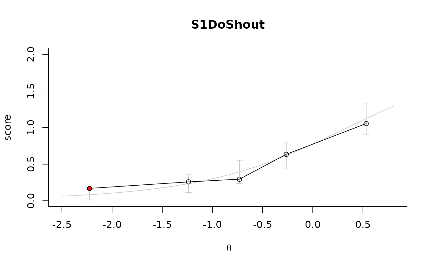
The plot shows 'fit' by comparing the expected score based on the model (grey line) with the average scores based on the data (black line with dots) for groups of students with similar estimated ability.

# S3 method for class 'enorm'
plot(
  x,
  item_id = NULL,
  dataSrc = NULL,
  predicate = NULL,
  nbins = 5,
  ci = 0.95,
  sort = c("none", "mse-desc", "mse-asc"),
  add = FALSE,
  col = "black",
  col.model = "grey80",
  ...
)

Arguments

x

object produced by fit_enorm

item_id

which item to plot, if NULL, one plot for each item is made

dataSrc

data source, see details

predicate

an expression to subset data in dataSrc

nbins

number of ability groups

ci

confidence interval for the error bars, between 0 and 1. Use 0 to suppress the error bars. Default = 0.95 for a 95% confidence interval

sort

for multiple items, sort item_id by mean squared error (i.e. the mean squared distance between the data and the model prediction per plot), either ascending (best to worst) or descending (worst to best). If none (the default) the order of items is not changed

add

logical; if TRUE add to an already existing plot

col

color for the observed score average

col.model

color for the expected score based on the model

...

further arguments to plot

Value

Silently, a data.frame with observed and expected values possibly useful to create a numerical fit measure.

Details

The standard plot shows the fit against the sample on which the parameters were fitted. If dataSrc is provided, the fit is shown against the observed data in dataSrc. This may be useful for plotting the fit in different subgroups as a visual test for item level DIF. The confidence intervals denote the uncertainty about the predicted pvalues within the ability groups for the sample size in dataSrc (if not NULL) or the original data on which the model was fit.

Examples

db = start_new_project(verbAggrRules, ":memory:", 
  person_properties=list(gender=""))

add_booklet(db, verbAggrData, "agg")
#> no column `person_id` provided, automatically generating unique person id's
#> $items
#>  [1] "S1DoCurse"   "S1DoScold"   "S1DoShout"   "S1WantCurse" "S1WantScold"
#>  [6] "S1WantShout" "S2DoCurse"   "S2DoScold"   "S2DoShout"   "S2WantCurse"
#> [11] "S2WantScold" "S2WantShout" "S3DoCurse"   "S3DoScold"   "S3DoShout"  
#> [16] "S3WantCurse" "S3WantScold" "S3WantShout" "S4DoCurse"   "S4DoScold"  
#> [21] "S4DoShout"   "S4WantCurse" "S4WantScold" "S4WantShout"
#> 
#> $person_properties
#> [1] "gender"
#> 
#> $columns_ignored
#> [1] "anger"
#> 

f = fit_enorm(db)

plot(f, item_id="S1DoShout")


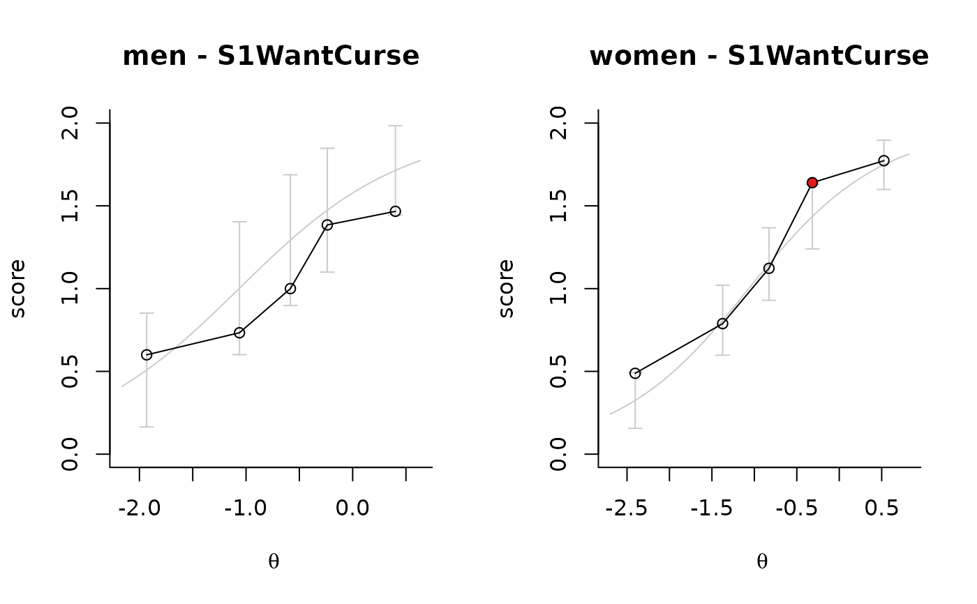
# side by side for two different groups
# (it is also possible to show two lines in the same plot 
# by specifying add=TRUE as an argument in the second plot)

par(mfrow=c(1,2))

plot(f,item_id="S1WantCurse",dataSrc=db, predicate = gender=='Male', 
  main='men - $item_id')

plot(f,items="S1WantCurse",dataSrc=db, predicate = gender=='Female', 
  main='women - $item_id')


close_project(db)